Efficient Management of Blockchain Data Capacity with StateDB Live Pruning

StateDB Live Pruning has been unveiled in Klaytn v1.11.0, promising efficient blockchain data capacity management.
Background
At the heart of blockchain data management lies the StateDB, responsible for holding a substantial portion of blockchain data, encompassing both account and storage trie information. The current StateDB mechanism involves continuously adding new nodes without altering existing node values. As the blockchain evolves, the Merkle Patricia Trie (MPT) handles changing data, causing shifts in intermediate nodes and leading to a surge of 6 to 10 trie nodes with every single node change. This has given rise to exponential growth in StateDB size over time. Despite attempts to alleviate this growth by eliminating historical data, the challenge of multi-reference issues among trie nodes has impeded efficient data pruning. As a result, the blockchain community has resorted to a method known as StateDB Offline Pruning, involving pausing, migrating, purging past data, lightening the StateDB with recent data, and rejoining as a blockchain node.
Introducing StateDB Live Pruning
StateDB Live Pruning addresses the hurdle of multiple node references in state trie through the strategic removal of hash duplication among state trie nodes. This approach effectively curtails data redundancy while maintaining the integrity of the existing MPT hashRoot by preserving its computational outcome. Consequently, the StateDB can be streamlined by erasing or relocating historical data to alternate storage, offering enhanced flexibility in storage utilization. This article delves into the specifics of trie node duplicate reference issues and how the StateDB Live Pruning feature triumphs over these challenges, enabling Live Pruning instead of Offline Pruning.
Understanding State Trie
Klaytn uses the Merkle Patricia Trie (MPT) for storing all account details in a tree structure. It is often referred to as the state tree, archived in Klaytn node storage. In Klaytn blockchain, each block features a state trie, responsible for storing account information. (Source: Klaytn v1.5.0 State Migration: Saving Node Storage)
For more information about state trie, see Ethereum State Trie Architecture Explained
The Challenge of Key Duplication in State Trie
The state trie of a blockchain typically adopts a key-value pairing, with each key pointing to another key in the value. These keys, typically 32-byte hashes of RLP-encoded results, result in hash redundancy when identical values are hashed. When a key is duplicated, only one instance occupies storage, yet multiple references within the state trie share the same data to economize storage space. However, this sharing obscures the scope of reference for each key, preventing their deletion and leading to data accumulation. Unfortunately, the storage savings from such sharing hovers around a mere 2%.
The Advent of Exthash
To tackle the key duplication challenge in state tries, the Exthash (extended hash) was developed.
- Conventional Hash: 32-byte Keccak256 hash
- Exthash: 32-byte Keccak256 hash + 7-byte serial index (nonce)
Exthash augments conventional hashes by appending a 7-byte serial index, generating a unique serial number for each hash iteration. This eliminates hash duplicates irrespective of preceding hash values.
Exthash’s Solution to Key Redundancy
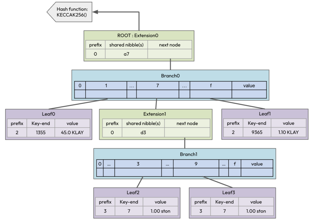
To illustrate Exthash’s efficacy, let’s employ an Ethereum-based example and the following account information. The MPT will be represented in both hash and Exthash forms.
a711355 : 45.0 KLAY
a77d337 : 1.00 ston
a7f9365: 1.10 KLAY
a77d397 : 1.00 ston
The hash representation below exhibits a problem with the last Leaf2, sharing identical information, referenced by two nodes.

Exthash representation, with added ExthashNonce shown in red, eradicates duplicate referenced nodes. Note that Leaf3, due to Exthash, introduces a new serial index.
Hashing Process using Exthash
Now, let’s take a step-by-step look at the process of creating an existing root hash using Exthash. Whereas Diagrams 1 and 2 earlier show the MPT after the hash calculation is completed, Diagram 3 below shows the MPT in memory before the hash is calculated.
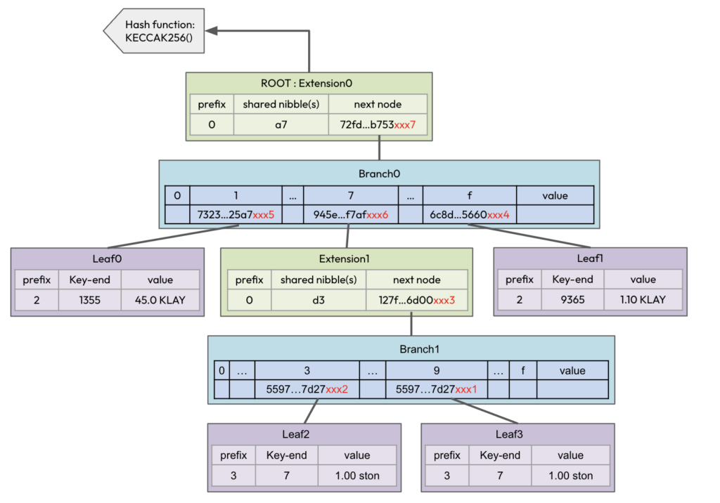
The sequence for obtaining an existing root hash entails a bottom-up hash calculation, commencing with the lowest node, that is, Leaf3.
- Leaf3 doesn’t have Exthash. So, you can just calculate the hash. The result will be “5597…7d27.” When you add the serial index “xxx1” to it, Leaf3’s Exthash becomes “5597…7d27xxx1.”
- Change child #9 of Branch1, which is connected to Leaf3, to “5597…7d27xxx1.”
- Leaf2 also uses the same hash calculation as Leaf3 but with a different serial index, that is “xxx2.” So, Leaf2’s Exthash will be “5597…7d27xxx2.”
- Change child #3 on Branch1 to “5597…7d27xxx2.”

5. Now, let’s compute the hash for Extension1. Within Branch1, two Exthashes are connected to Extension1. To calculate the hash, we will remove the two serial indices of Exthashes temporarily (“5597…7d27xxx1,” …, “5597…7d27xxx2,” … → “5597…7d27,” …, “5597…7d27,” …) and calculate the hash, resulting in “127f…6d00.” Here, adding the serial index “xxx3” to it produces “127f…6d00xxx3.”

6. Since Leaf1 and Leaf0 don’t use Exthash, so we can calculate their hashes directly. The calculated values include the serial indices xxx4 and xxx5 respectively. For Leaf1, it’s “6c8d…5660xxx4,” and for Leaf0, it’s “6c8d…5660xxx5.”
7. The value “127f…6d00xxx3” is in Exthash format. Following the previous pattern, after removing the serial index and computing the hash (“945e…f7af”), we’ll obtain the value with the serial index xxx6 (“945e…f7afxxx6”).
8. Finally, if we apply the same process to Branch0 and Extension0 as we did for Branch1 and Extension1, we will achieve the same outcome as shown in Diagram-2. This process will lead us to the same root hash as demonstrated in Diagram-1, ensuring compatibility.
Pruning Process using Exthash
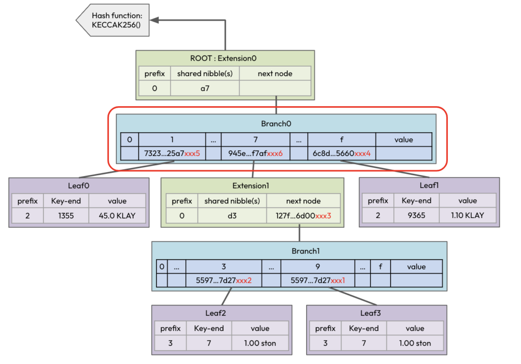
Let’s explain the process of pruning a node with the Exthash method.
Pruning using hash
First, we’ll remove the MPT node organized with hash.
- If we represent Diagram-1 in the format of key and value pairs, it will appear as follows:
Extension0 - acec...e3c5 : [ "a7", "72fd...b753" ]
Branch0 - 72fd...b753 : [ 0:N, 1:"7323...25a7", 2:N, ..., 7:"945e...f7af", 8:N, ..., f:"6c8d...5660", val ]
Leaf0 - 7323...25a7 : [ "1355", 45.0 KLAY ]
Extension1 - 945e...f7af : [ "d3", "127f...6d00" ]
Leaf1 - 6c8d...5660 : [ "9365", 1.10 KLAY ]
Branch1 - 127f...6d00 : [ 0:N, ..., 3:"5597...7d27", ..., 9:"5597...7d27", ..., f:N, val ]
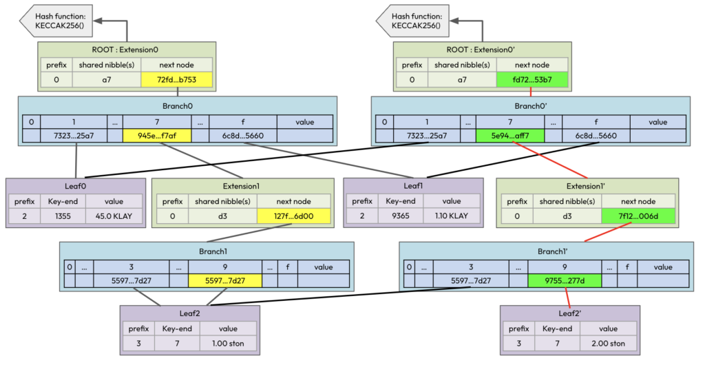
Leaf2 - 5597...7d27 : [ "7", 1.00 ston ]2. If the balance of the account a77d397 changes from 1.00 STON to 2.00 STON, Diagram-1 will transform into Diagram-7 shown below. The nodes with a light green background are the newly updated nodes.
3. Let’s represent Diagram-7 in the key : value format.
Extension0 - acec...e3c5 : [ "a7", "72fd...b753" ]
Branch0 - 72fd...b753 : [ 0:N, 1:"7323...25a7", 2:N, ..., 7:"945e...f7af", 8:N, ..., f:"6c8d...5660", val ]
Leaf0 - 7323...25a7 : [ "1355", 45.0 KLAY ]
Extension1 - 945e...f7af : [ "d3", "127f...6d00" ]
Leaf1 - 6c8d...5660 : [ "9365", 1.10 KLAY ]
Branch1 - 127f...6d00 : [ 0:N, ..., 3:"5597...7d27", ..., 9:"5597...7d27", ..., f:N, val ]
Leaf2 - 5597...7d27 : [ "7", 1.00 ston ]
Leaf2' - REDD...7d27 : [ "7", 2.00 ston ]
Branch1' - REDD...6d00 : [ 0:N, ..., 3:"5597...7d27", ..., 9:"9755...277d", ..., f:N, val ]
Extension1'- REDD...f7af : [ "d3", "7f12...006d" ]
Branch0' - REDD...b753 : [ 0:N, 1:"7323...25a7", 2:N, ..., 7:"5e94...aff7", 8:N, ..., f:"6c8d...5660", val ]
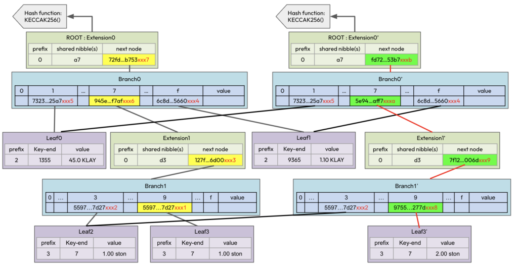
Extension0'- REDD...e3c5 : [ "a7", "fd72...53b7" ]4. When it comes to pruning, the nodes marked with a prime (‘) symbol (for example, Leaf2′, Branch1′, etc.) are the updated nodes. These nodes should be removed along with their previous versions. However, deleting Leaf2, which is the source node for Leaf2’, would result in data loss since Branch1 was referring to Leaf2 as a duplicate. This is a simplified example. In a large MPT with billions of connected nodes, it’s challenging to determine which nodes are eligible for deletion when new updates are applied. As a result, live purging is not feasible.
Pruning using Exthash
Now, let’s proceed to delete the MPT node using the Exthash method.
- If we represent Diagram-1 using key-value pairs, it will look like this:
Extension0 - acec...e3c5 : [ "a7", "72fd...b753" ]
Branch0    - 72fd...b753 : [ 0:N, 1:"7323...25a7", 2:N, ..., 7:"945e...f7af", 8:N, ..., f:"6c8d...5660", val ]
Leaf0      - 7323...25a7 : [ "1355", 45.0 KLAY ]
Extension1 - 945e...f7af : [ "d3", "127f...6d00" ]
Leaf1      - 6c8d...5660 : [ "9365", 1.10 KLAY ]
Branch1    - 127f...6d00 : [ 0:N, ..., 3:"5597...7d27", ..., 9:"5597...7d27", ..., f:N, val ]
Leaf2      - 5597...7d27 : [ "7", 1.00 ston ]

Leaf2'     - REDD...7d27 : [ "7", 2.00 ston ]
Branch1'   - REDD...6d00 : [ 0:N, ..., 3:"5597...7d27", ..., 9:"9755...277d", ..., f:N, val ]
Extension1'- REDD...f7af : [ "d3", "7f12...006d" ]
Branch0'   - REDD...b753 : [ 0:N, 1:"7323...25a7", 2:N, ..., 7:"5e94...aff7", 8:N, ..., f:"6c8d...5660", val ]
Extension0'- REDD...e3c5 : [ "a7", "fd72...53b7" ]
2. If the balance of the account a77d397 changes from 1.00 STON to 2.00 STON, Diagram-2 will transform into Diagram-8 shown below. The Exthash associated with a77d397 is recalculated and represented by the light green box.
3. Let’s represent Diagram-8 using key-value pairs.
Extension0 - acec...e3c5 : [ "a7", "72fd...b753" ]
Branch0    - 72fd...b753 : [ 0:N, 1:"7323...25a7", 2:N, ..., 7:"945e...f7af", 8:N, ..., f:"6c8d...5660", val ]
Leaf0      - 7323...25a7 : [ "1355", 45.0 KLAY ]
Extension1 - 945e...f7af : [ "d3", "127f...6d00" ]
Leaf1      - 6c8d...5660 : [ "9365", 1.10 KLAY ]
Branch1    - 127f...6d00 : [ 0:N, ..., 3:"5597...7d27", ..., 9:"5597...7d27", ..., f:N, val ]
Leaf2      - 5597...7d27 : [ "7", 1.00 ston ]

Leaf2'     - REDD...7d27 : [ "7", 2.00 ston ]
Branch1'   - REDD...6d00 : [ 0:N, ..., 3:"5597...7d27", ..., 9:"9755...277d", ..., f:N, val ]
Extension1'- REDD...f7af : [ "d3", "7f12...006d" ]
Branch0'   - REDD...b753 : [ 0:N, 1:"7323...25a7", 2:N, ..., 7:"5e94...aff7", 8:N, ..., f:"6c8d...5660", val ]
Extension0'- REDD...e3c5 : [ "a7", "fd72...53b7" ]
4. Since the balance of Leaf3 has changed, Leaf3, Branch1, Extension1, Branch0, and Extension0 have been updated to Leaf3′, Branch1′, Extension1′, Branch0′, and Extension0′ respectively. In addition to updating the data, historical nodes like Leaf3, Branch1, Extension1, Branch0, and Extension0 can be safely deleted because the added 7 bytes ensure the absence of duplicate referencing nodes. The nodes with identifiers “5597…7d27xxx1”, “127f…6d00xxx3”, “945e…f7afxxx6”, “72fd…b753xxx7”, and “acec…e3c5” are all deleted, completing the live pruning process.
Implications of StateDB Live Pruning for Nodes
By using StateDB Live Pruning, the StateDB retains only the most recent two days of state data (172,800 blocks by default), discarding earlier state data. This results in a compact StateDB, ranging from 150 to 200 GB approximately. This boosts IO performance by elevating storage-related cache hit ratios.
Although historical data deletion entails the introduction of a delete queue and potential system load increase due to key-value deletion processes, monitoring reveals no discernible rise in load. This is potentially offset by enhanced IO performance.
Enabling StateDB Live Pruning for Node Operation
As StateDB Pruning incorporates the new Exthash type, DB migration is achievable only through existing archive sync and full sync methods. However, the significantly reduced DB capacity eases download and synchronization processes. In fact, the discrepancy between downloaded data size using snap sync or fast sync and StateDB Pruned DB size is negligible. You can follow the docs to enable the StateDB Live Pruning feature.
What’s Next for StateDB Live Pruning
Consensus nodes (CN) and proxy nodes (PN) are ideal candidates for StateDB Live Pruning due to their primary function of synchronizing and validating the latest data.
However, endpoint nodes (EN), which handle diverse API requests, may not benefit significantly. Therefore, we’re contemplating a StateDB migration technique that transfers historical data to alternative storage rather than erasing it. The goal is to optimize storage costs by utilizing high-performance hot storage for recent data and more expansive but slower cold storage for older information.
Additionally, the option to further strip information like headers, bodies, receipts, etc. is in development, intended to enhance node performance efficiency.